Linear Regression - Theory, Implementation and Analysis | Portfolio de Mateo

Linear regression is one of the most fundamental mathematical models in machine learning of AI models, despite its simplicity, it is a very important technique to understand the relationships between variables and serves as a base for understanding and operating more complex models.

In this article we will look at different models and techniques related to the central theme of the article:

Practical applications

Price prediction (housing, stocks, etc.)
Trend estimation
Relationships between variables in scientific studies

Why is it essential to know what linear regression is to get started with AI?

Learning what linear regression is and its essence is one of the first recommended steps to get started in the world of artificial intelligence and machine learning. Let’s see why from four key perspectives:

✅ 1. Establishes the foundations of supervised learning:

Linear regression is the simplest supervised learning model.
Provides an understanding of how a model learns to recognize patterns from labeled data.
Introduces the concept of a loss function, which measures how well the model is learning.
Teaches the idea of generalization = applying learning to new data.

✅ 2. Introduces key mathematical concepts:

Defines mathematical functions to measure errors (such as the Mean Square Error, MSE).
Allows you to study basic calculus such as derivatives and gradient descent to optimize models.
Facilitates the use of linear algebra (vectors, matrices), which is key in complex models.

✅ 3. Direct connection with neural networks:

Imagine a neural network as several “layers” that process data, if you only have one layer that does simple addition and multiplication (no complicated stuff), that is just a linear regression.
Logistic regression is almost the same, but after that sum, we apply a function that converts the result into a probability (sigmoid).
Some ideas for preventing the model from being confused by the data (such as Ridge and Lasso) come from linear regression and are also used in larger neural networks.

We will see all this in future articles :)

✅ 4. Applicable to practice from day one:

You can quickly apply linear regression to real datasets.
Typical examples: housing price prediction, salary estimation, or sales analysis.
It is used to validate ideas and generate agile prototypes in AI projects.

Problem statement

Given a data set with an explanatory variable $X$ and a target variable $Y$, we want to find a linear relationship that allows us to predict the value of $Y$ from $X$ using a simple formula:

$\begin{equation} \hat{y} = wx + b \end{equation}$

Where:

$w$ (slope or coefficient): represents how much the target variable $Y$ changes when the explanatory variable $X$ increases by one unit.
- For example, if $w = 2$, it means that for every increase of 1 in $X$, $Y$ will increase by approximately 2.
$b$ (independent term or bias): is the value that $Y$ takes when $X = 0$.
It is the point where the regression line crosses the vertical axis ($Y$ axis) and adjusts the line to better fit the data.
$\hat{y}$ (prediction): is the estimated or calculated value of $Y$ for a given value of $X$, it is the output that the model gives us to make predictions.

Practical Understanding

Imagine you want to predict the price of a house based on its size (in square meters). In this case:

$w$ is the coefficient that indicates how much the price increases for each additional square meter.
- For example, if $w = $1,500$, it means that each additional square meter increases the price by €1,500.
$b$ is the base price, that is, the estimated price of a house with a size of 0 (conceptually the starting point).
- For example, if $b = $50,000$, that would be the minimum or base cost of the house regardless of the size.
$\hat{y}$ is the price prediction for a specific size.

For example, if you have a house of 100 square meters:

$\begin{equation} \hat{y} = 1{,}500 \cdot 100 + 50{,}000 = 150{,}000 + 50{,}000 = 200{,}000 \end{equation}$

The model predicts that the approximate price will be €200,000.

Relationship with neural networks

This linear regression model can be seen as a very simple neuron in a neural network, where:

The input is the value $x$ (size of the house).
The weight $w$ multiplies that input to adjust its importance.
The bias $b$ is added to shift the output and improve the fit.
There is no activation function, so the output is simply a linear combination.

That is, this neuron directly calculates the predicted value without transforming it, which is exactly what linear regression does.

This understanding helps to see that more complex models, such as deep neural networks, are built from many similar layers and neurons, but with activation functions that allow them to learn non-linear relationships.

Loss Function: Mean Square Error (MSE)

The loss function tells us how well or poorly our model is performing, comparing the predictions with the actual values.

It’s simple, we need to know if our predictions are close to reality or are complete nonsense and with that information we can improve the accuracy of the model.

For linear regression we use a function called Mean Square Error (MSE), which is calculated like this:

$\begin{equation} MSE = \frac{1}{n} \sum_{i=1}^n (y_i - \hat{y}_i)^2 \end{equation}$

Explanation

We compare each actual value $y_i$ with its prediction $\hat{y}_i$.
We subtract to see the difference (error).
We square that difference so that the larger errors weigh more.
We take the average of all those squared errors.

Thus, if our predictions are very far from the actual values, the MSE will be large; if they are close, it will be small.

Why is it useful?

The objective of the model is to make the MSE as small as possible, that is, to make the predictions as close to the real values as possible.

Practical application:

Returning to the house example, imagine we want to predict the price of a house based on its size.

Let’s say the house is 100 square meters.
Our model predicts that the price will be €150,000.
But the actual price is €160,000.

The error is the difference between the actual and predicted price:

$\begin{equation} 160{,}000 - 150{,}000 = 10{,}000 \end{equation}$

We square this error so that large errors carry more weight:

$\begin{equation} 10{,}000^2 = 100{,}000{,}000 \end{equation}$

If we do this for many houses and then take the average, we get the MSE.

The smaller this number, the better our model is because it means our predictions are close to actual prices.

Therefore, in practice, when training a model, we try to minimize the MSE so that our predictions are as accurate as possible.

Relationship with neural networks

In neural networks, this loss function is also used to determine how well they are performing and to tune the numbers that control the model (the weights and biases).

Minimizing the MSE is like saying “I want my model to make as few errors as possible”.

Analytical solution (closed-form)

When we have our data, we can directly calculate the slope $w$ and the intercept $b$ of the best line that fits that data without having to do many tests.

The formulas are:

$\begin{equation} w = \frac{\sum (x_i - \bar{x})(y_i - \bar{y})}{\sum (x_i - \bar{x})^2} \end{equation}$

$\begin{equation} b = \bar{y} - w \bar{x} \end{equation}$

Where $\bar{x}$ y $\bar{y}$, these are the averages of all house sizes and prices.

Practical intuition

This method finds in a single step the line that best fits all the data, minimizing the sum of the squared errors.

Practical application with the example of the house

Imagine you have data for several houses with their sizes and prices:

Size (m²)	Price (€)
80	120000
100	150000
120	180000

The method calculates how much the average price changes when the average size changes (that’s $w$), and what the base price is when the size is zero (that’s $b$).

With these values, you can predict the price of a new home just by knowing its size.

Python Implementation

  
import numpy as np

def linear_regression_analytic(x, y):
    x_mean, y_mean = np.mean(x), np.mean(y)
    w = np.sum((x - x_mean) * (y - y_mean)) / np.sum((x - x_mean)**2)
    b = y_mean - w * x_mean
    return w, b

x = np.array([80, 100, 120])          # Sizes
y = np.array([120000, 150000, 180000])  # Prices

w, b = linear_regression_analytic(x, y)
print(f"Slope (w): {w}")
print(f"Intercept (b): {b}")

Result:

  
Slope (w): 1500.0 
Intercept (b): 0.0

Slope (w) = 1,500.0

This means that for every additional square meter in the house’s size, the price

increases by 1,500 €.

For example, if a house is 10 m² larger, the price will increase by approximately €15,000 (10 × 1,500 €).

Intercept (b) = 0

This value is the base price when the house size is 0 m², in this case, it’s 0 €, which makes sense because a house with no size would have no price.

In other cases, the intercept may be different and adjust the prediction line.

So the prediction formula would be:

$\begin{equation} \hat{y} = 1{,}500 \cdot x + 0 \end{equation}$

So, if you want to predict the price of a 90 m² house, you just have to multiply:

$\begin{equation} \hat{y} = 1{,}500 \cdot 90 = 135{,}000 \, \text{€} \end{equation}$

5. Gradient descent

When we have a lot of data or several variables, using the direct formula can be complicated or very slow, so we use gradient descent, which gradually adjusts the parameters to improve the prediction.

This method allows us to gradually adjust the parameters (slope and bias) of the line until the error is as small as possible.

Formulas to apply

These formulas tell us how to change w and b to improve the model, by calculating the slope of the error:

$\begin{equation} \frac{\partial \text{MSE}}{\partial w} = -\frac{2}{n} \sum x_i (y_i - \hat{y}_i) \end{equation}$

$\begin{equation} \frac{\partial \text{MSE}}{\partial b} = -\frac{2}{n} \sum (y_i - \hat{y}_i) \end{equation}$

Step-by-step algorithm

We start with w and b equal to zero (or any value).
We calculate the predictions with those values.
We measure the error between the predictions and the actual values.
We calculate how much w and b need to change to reduce that error (gradients).
We update w and b slightly in the direction that reduces the error.
We repeat this many times until the error is minimal or changes little.

Python Implementation

  
def gradient_descent(x, y, lr=0.01, epochs=1000):
    n = len(x)
    w, b = 0.0, 0.0
    for _ in range(epochs):
        y_pred = w * x + b
        error = y - y_pred
        dw = -2 * np.dot(x, error) / n
        db = -2 * np.sum(error) / n
        w -= lr * dw
        b -= lr * db
    return w, b

$w$ = 2.18, meaning that for each additional square meter the house has, the price increases approximately 2.18 € thousand
$b$ = 10.24 thousand € is the base price value when the house has 0 square meters, although in real life a house with 0 m² does not make sense, this value serves as a starting point for the regression line.

The formula to predict the price is:

$\begin{equation} \text{precio} = 2.18 \times m^2 + 10.24 \end{equation} $

So, if a house is 50 m², its estimated price would be:

$\begin{equation} 2.18 \times 50 + 10.24 = 119.24 \text{ thousands of €} \end{equation}$

Practical application (house price example)

If we start with $w = 0$ and $b = 0$, the model always predicts 0 € regardless of size, using gradient descent, each step adjusts the base price $b$ and how much the price per square meter $w$ increases to get closer to the actual price of the houses.

Relationship with neural networks

This process of adjusting parameters step by step is exactly what neural networks do when trained with backpropagation

We will also explain this in future posts.

Linear regression is the simplest way to apply this idea.

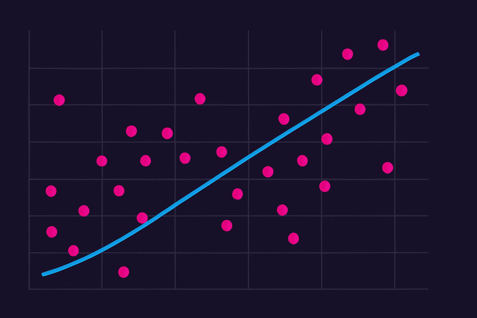
Visualization

Viewing the data and the regression line on a graph helps us understand how the model works.

By comparing the line with the points, we can see if the model is making good predictions or if it is far from the real data, this visualization is a practical tool to interpret and validate the model.

  
x = np.array([45, 50, 55, 60, 65, 70, 75, 80, 85, 90, 95, 100, 110, 120, 130, 140, 150, 160, 170, 180])
y = np.array([90, 95, 100, 115, 120, 125, 135, 140, 150, 160, 165, 175, 190, 210, 220, 240, 255, 265, 280, 300])

N = len(x)
sum_x = np.sum(x)
sum_y = np.sum(y)
sum_xy = np.sum(x * y)
sum_x2 = np.sum(x ** 2)

w = (N * sum_xy - sum_x * sum_y) / (N * sum_x2 - sum_x**2)
b = (sum_y / N) - w * (sum_x / N)

def predict(x):
    return w * x + b

plt.scatter(x, y, label="Data")
plt.plot(x, predict(x), color="red", label=f"Regression (w={w:.2f}, b={b:.2f})")
plt.xlabel("m2")
plt.ylabel("Price (thousands €)")
plt.legend()
plt.show()

Code and graphic explanation

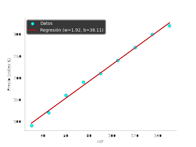
Blue dots (scatter): represent the actual data, houses with their size and price.
Red line (plot): the line that best fits the data according to the linear regression.
The slope $w$ tells us how much the price increases for each additional square meter.
The intercept $b$ is the estimated price for a house with size 0.
The graph shows how the model predicts the price based on the house’s size.

Relationship with complex models

A neural network with a single linear layer is basically a linear regression.
Logistic regression is similar, but applies a sigmoid function to the output to solve classification problems (deciding between categories).
Techniques such as Ridge (L2) and Lasso (L1) are forms of regularization that help prevent the model from fitting too much to the training data (overfitting), these techniques are used both in linear regression and in more complex neural networks.

We will see what a sigmoid function is in the future

Conclusion

In this article we have covered:

The theory and mathematics underlying linear regression.
Two ways to solve it: analytical solution and gradient descent.
Practical implementations in Python.
Visualization to understand the model.
Key connections with neural networks and their importance in AI.

I hope you enjoyed reading this article as much as I did. Thanks for reading!